NOTE: This information is taken from Prof. Jerry Reiter’s website for his Stat 210 course at Duke University.
The television series Sesame Street is concerned mainly with teaching preschool skills to children age 3-5, with special emphasis on reaching economically disadvantaged children. The show is designed to hold young childrens’ attention through action oriented, short duration presentations teaching specific preschool cognitive skills and some social skills. Each show is one hour and involves much repetition of concepts within and across shows.
Does Sesame Street help economically disadvantaged children ‘catch-up’ with economically advantaged children? In the early 1970s, researchers at Educational Testing Service (the company that runs the SAT) ran a study to evaluate Sesame Street. The researchers sampled children representative of economically advantaged and disadvantaged populations from five different sites in the United States. To ensure the study contained a group of children that watched Sesame Street regularly, they randomly assigned children either to receive encouragement to watch Sesame Street or not to receive encouragement. Those assigned to encouragement were given promotional materials, and received weekly visits and phone calls from ETS staff. Those assigned not to receive encouragement did not get this attention. The children were tested on a variety of cognitive variables, including knowledge of body parts, knowledge about letters, knowledge about numbers, etc., both before and after viewing the series.
These data, available here as a CSV file, are part of a larger data set used to evaluate the impact of Sesame Street. The names of variables are shown in the code book below.
- id : subject identification number
- site :
1 =Three to five year old disadvantaged children from inner city areas in various parts of the country. 2 = Four year old advantaged suburban children. 3 = Advantaged rural children. 4 = Disadvantaged rural children. 5 = Disadvantaged Spanish speaking children. - sex male=1, female=2
- age age in months
- viewcat frequency of viewing 1=rarely watched the show 2=once or twice a week 3=three to five times a week 4=watched the show on average more than 5 times a week
- setting: setting in which Sesame Street was viewed, 1=home 2=school
- viewenc : treatment condition 1=child encouraged to watch, 2=child not encouraged to watch
- prebody : pretest on knowledge of body parts (scores range from 0-32)
- prelet : pretest on letters (scores range from 0-58)
- preform : pretest on forms (scores range from 0-20)
- prenumb : pretest on numbers (scores range from 0-54)
- prerelat : pretest on relational terms (scores range from 0-17)
- preclasf : pretest on classification skills
- postbody : posttest on knowledge of body parts (0-32)
- postlet : posttest on letters (0-58)
- postform : posttest on forms (0-20)
- postnumb : posttest on numbers (0-54)
- postrelat : posttest on relational terms (0-17)
- postclasf: posttest on classification skills
- peabody: mental age score obtained from administration of the Peabody Picture Vocabulary test as a pretest measure of vocabulary maturity. Taken before the experimental intervention.
- numbers: postnumb - prenumb. Variable constructed by Prof. Reiter.
- letters: postlet - prelet. Variable constructed by Prof. Reiter.
- num.let: numbers - letters. Variable constructed by Prof. Reiter.
[The following is not from Prof. Reiter]
Example of access
file_url <- "https://raw.githubusercontent.com/matackett/intro-regression/master/data/sesame.csv"
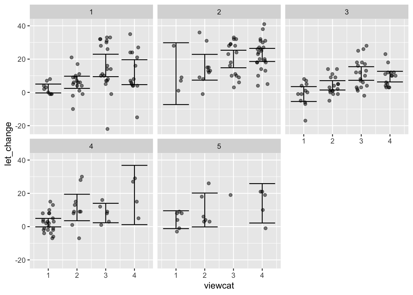
Sesame <- readr::read_csv(file_url)Suppose we want to look at the increase in test scores on letters as a function of how much the child watched Sesame street. prelet and postlet are the before-and-after test scores, viewcat is how often the child watched the show.
library(dplyr)
library(mosaic)
Tmp <-
  Sesame  %>%
  mutate(let_change = postlet - prelet)
Stats <- df_stats(let_change ~ viewcat + site, data = Tmp, ci.mean(.95))

Stats
## viewcat site lower upper
## 1 1 1 -0.3294109 4.996078
## 2 2 1 2.4029558 9.714691
## 3 3 1 9.4611400 22.938860
## 4 4 1 4.6561841 19.629530
## 5 1 2 -7.3237393 29.823739
## 6 2 2 7.3552542 22.844746
## 7 3 2 14.7919881 25.325659
## 8 4 2 18.5623775 26.437622
## 9 1 3 -5.4681691 3.468169
## 10 2 3 1.4219269 7.048661
## 11 3 3 7.2607019 15.439298
## 12 4 3 6.2726063 12.660727
## 13 1 4 -0.1528044 4.935413
## 14 2 4 3.5466237 19.453376
## 15 3 4 2.3267986 14.006535
## 16 4 4 1.1858796 36.814120
## 17 1 5 -1.2015497 9.534883
## 18 2 5 -0.1746560 20.174656
## 19 3 5 NaN NaN
## 20 4 5 2.1552804 25.844720Tmp %>%
gf_jitter(let_change ~ viewcat | site, width = 0.2, height = 0, alpha = .50) %>%
gf_errorbar(lower + upper ~ viewcat | site, data = Stats)