We almost always work with variables that are either …
- quantitative
- categorical with only two levels
In relating two variables, there are four possible situations
| Quantitative | Categorical | |
|---|---|---|
 |
 |
|
| Quant. | slope of regression line or correlation coefficient | difference in two means |
| …………. | …………………………………… | ………………………………………. |
| Categ. | ?????? | difference in two proportions |
Presentation in terms of algebra
| Quantitative | Categorical | |
|---|---|---|
 |
 |
|
| Quant. | \(b_1 = \frac{n\sum xy - \sum x \cdot \sum y}{n \sum x^2 - (\sum x)^2}\) | \(t = \frac{\bar{x}_1 - \bar{x}_2 - (\mu_1 - \mu_2)}{\sqrt{\frac{s_p^2}{n_1} + \frac{s_p^2}{n_2}}}\) |
| …………. | …………………………………… | ………………………………………. |
| Categ. | ?????? | \(z = \frac{(\hat{p_1} - \hat{p_2}) - (p_1 - p_2)}{\sqrt{\frac{\bar{p}\bar{q}}{n_1} + \frac{\bar{p}\bar{q}}{n_2}}}\) |
… and associated distributions: t and z
Data beats formulas
| Quantitative | Categorical | |
|---|---|---|
 |
 |
|
| Quant. | 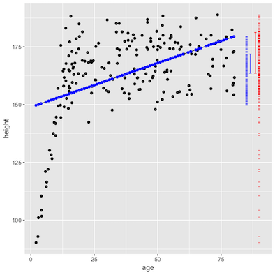 |
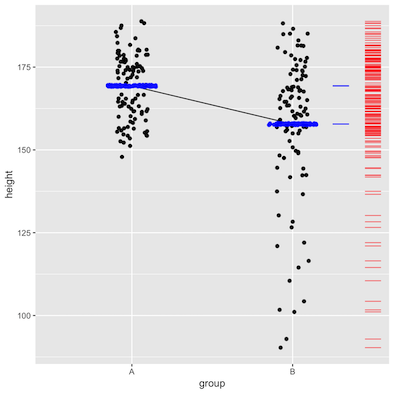 |
| …………. | …………………………………… | ………………………………………. |
| Categ. | 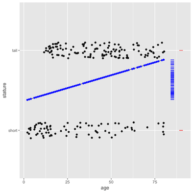 |
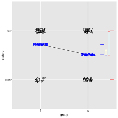 |
Raw and model values
The error bars show the size of the standard deviation.
knitr::include_graphics("/images/PQQ.png")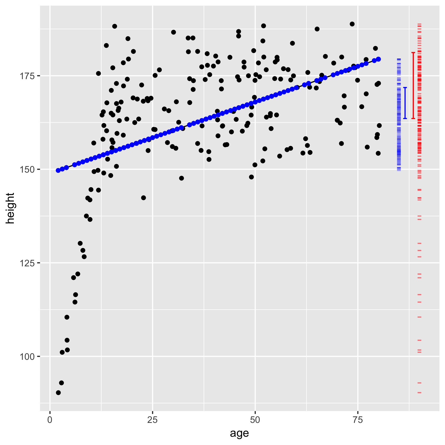
The formal inference procedure
- Measure the effect size. Call it \(\beta\):
- slope for Quant vs Quant or Cat vs Quant
- difference for Quant vs Cat or Cat vs Cat
- Take the ratio of the model-value standard deviation to the raw-value standard deviation. Call this ratio \(R\).

- Compute the ratio of “explained” to “unexplained”: \[F = (n-1) \frac{R^2}{1 - R^2}\]
Eyeballing from the four models (which had n = 200)…
| Quantitative | Categorical | |
|---|---|---|
| Quantitative | \(\beta = \frac{1\ cm}{3\ years}\) \(R \approx 0.5\) \(F = 24.8\) | \(\beta \approx 8\ cm\), \(R \approx 1/3\) \(F \approx 66\) |
| Categorical | \(\beta = 0.007\) per year, \(R \approx 0.12\) \(F \approx 8.3\) | \(\beta \approx 0.2\), \(R \approx 0.25\) \(F \approx 13.3\) |
Confidence interval on \(\beta\) is always \[CI_\beta = \beta (1 \pm 2 / \sqrt{F})\]
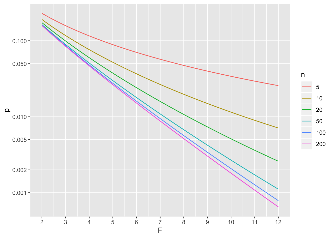
p-value … Look up in this graph.
Freebies:
- correlation coefficient \(r = \sqrt{F}\), where the \(\pm\) branch is based on the slope.
- Prefer t? It’s \(t = \sqrt{F}\). But F is more general than t.